Exploring the Iris Dataset with Python

The Iris dataset is one of the most famous datasets in the field of machine learning and data science. Introduced by the British biologist and statistician Ronald A. Fisher in 1936, it remains a popular choice for beginners exploring data analysis and machine learning. This blog post will take you through the basics of the Iris dataset, from understanding its structure to performing basic analysis and visualization.

What is the Iris Dataset?

The Iris dataset consists of 150 samples from three different species of iris flowers: Iris setosa, Iris versicolor, and Iris virginica. Each sample has four features:

1. Sepal length (cm)

2. Sepal width (cm)

3. Petal length (cm)

4. Petal width (cm)

These features describe the physical dimensions of the flowers. Additionally, each sample is labeled with the species it belongs to, making this a labeled dataset suitable for supervised learning tasks.

Loading Iris Dataset with Python

The Iris dataset, accessible via the sklearn.datasets module in the scikit-learn library, is a classic dataset widely used for machine learning and data analysis. It consists of 150 samples from three species of iris flowers (Iris setosa, Iris versicolor, and Iris virginica), with each sample containing four numeric features: sepal length, sepal width, petal length, and petal width. The dataset is well-suited for classification tasks due to its balanced and labeled nature. In scikit-learn, the dataset can be easily loaded using the load_iris function, which provides the data in a structured format including the feature matrix and target labels. This ease of access makes the Iris dataset an ideal choice for beginners looking to practice data preprocessing, visualization, and machine learning techniques. Here's a simple example of how to load the dataset using scikit-learn:

from sklearn.datasets import load_iris

import pandas as pd

# Load the iris dataset

iris = load_iris()

# Create a DataFrame

df = pd.DataFrame(data=iris.data, columns=iris.feature_names)

df['species'] = iris.target

# Map target integers to species names

df['species'] = df['species'].map({0: 'setosa', 1: 'versicolor', 2: 'virginica'})

df.head()

Output for the above code:

Exploratory Data Analysis (EDA) in Python

Before diving into machine learning, it's essential to understand the dataset through exploratory data analysis. EDA helps in identifying patterns, detecting outliers, and uncovering insights.

1. Descriptive Statistics

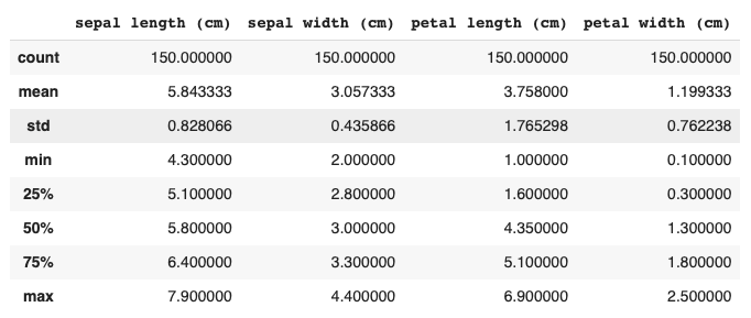
Descriptive statistics provide a summary of the dataset, including mean, median, standard deviation, and other metrics. Here's how you can calculate these statistics:

# Descriptive Statistics

df.describe()

Output for the above code:

2. Visualizing the Data

Visualization is a powerful tool for EDA. Let's explore some basic plots:

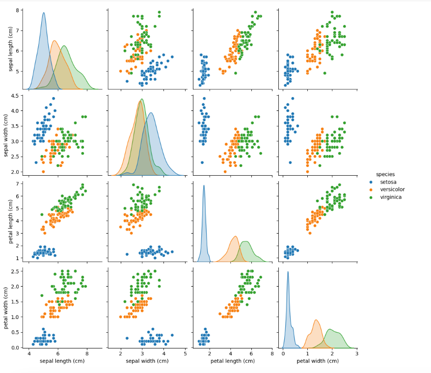
Pair Plot A pair plot visualizes the pairwise relationships between features. It's useful for understanding how different features interact with each other.

import seaborn as sns

import matplotlib.pyplot as plt

sns.pairplot(df, hue='species')

plt.show()

Output for the above code:

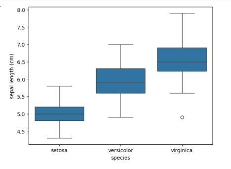
Box Plot Box plots display the distribution of data based on quartiles and can help identify outliers.

sns.boxplot(x='species', y='sepal length (cm)', data=df)

plt.show()

Output for the above code:

Bar Plot: Displays the distribution of target classes

df.groupby('species').size().plot(kind='barh', color=sns.palettes.mpl_palette('Dark2'))

plt.gca().spines[['top', 'right',]].set_visible(False)

Output for the above code:

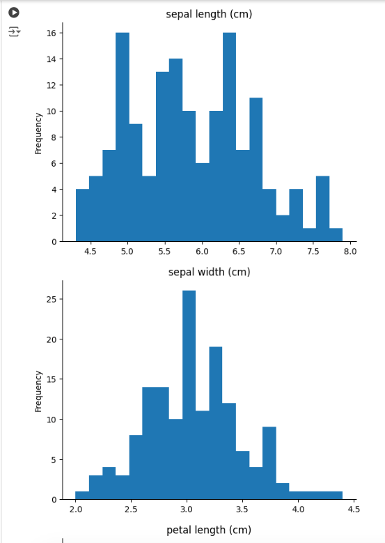
Histogram: Shows distribution of different features

for col in df.columns:

  try:

     df[col].plot(kind='hist', bins=20, title=col)

     plt.gca().spines[['top', 'right',]].set_visible(False)

     plt.show()

  except:

     print('non numeric data')

Output for the above code:

Similar plots for other features will also be displayed.

Applying Machine Learning Models

The Iris dataset, a staple in the world of data science and machine learning, offers a perfect starting point for beginners to learn about data analysis with Python. Utilizing Python libraries like pandas and scikit-learn, one can easily load and explore the dataset, perform descriptive statistics, and visualize data through plots. By applying machine learning algorithms such as the k-Nearest Neighbors (k-NN) classifier, users can predict the species of an iris flower with impressive accuracy, illustrating the practical applications of data analysis and machine learning. This hands-on experience with the Iris dataset provides foundational skills that are essential for tackling more complex datasets and problems in the field of data science. The Iris dataset is often used for classification tasks, where the goal is to predict the species of a flower based on its features. Let's apply a simple machine learning model: the k-Nearest Neighbors (k-NN) classifier.

1. Data Preprocessing

First, we need to split the dataset into training and testing sets.

from sklearn.model_selection import train_test_split

X = df.drop('species', axis=1)

y = df['species']

X_train, X_test, y_train, y_test = train_test_split(X, y, test_size=0.3, random_state=42)

2. Training the Model

from sklearn.neighbors import KNeighborsClassifier

# Initialize the model

knn = KNeighborsClassifier(n_neighbors=3)

# Train the model

knn.fit(X_train, y_train)

3. Evaluating the Model

from sklearn.metrics import accuracy_score

# Predict the species for the test set

y_pred = knn.predict(X_test)

# Calculate the accuracy

accuracy = accuracy_score(y_test, y_pred)

print(f"Accuracy: {accuracy}")

Output for the above code:

Accuracy: 1.0

The accuracy score provides a measure of how well the model performs. For the Iris dataset, k-NN often achieves high accuracy due to the clear separation between classes.

In conclusion, the Iris dataset is a fantastic starting point for anyone new to data science and machine learning. Through this blog, we've covered the basics of loading the dataset, performing exploratory data analysis, and applying a simple classification model. As you gain more experience, you can explore other machine learning models and techniques to further improve accuracy and insights.

Remember, the key to becoming proficient in data science is practice. So, keep experimenting with different datasets, models, and techniques!