
Support Vector Machine (SVM) is a powerful classification algorithm widely used in machine learning for its ability to handle complex datasets and perform well in high-dimensional spaces. In this blog, we'll explore the Iris dataset, a classic dataset for pattern recognition, and implement an SVM model to classify iris flowers into three different species based on their features.
What is the Support Vector Machine (SVM) Algorithm?
Support Vector Machine (SVM) is a supervised learning algorithm used primarily for classification tasks, though it can also be applied to regression problems. SVM works by finding the optimal hyperplane that separates data points of different classes in a feature space. The goal is to identify the hyperplane that maximizes the margin, or the distance, between the closest data points of each class. These closest points are known as support vectors. By focusing on these critical points, SVM aims to create the best possible boundary that generalizes well to unseen data. SVM is highly valued in the machine learning community due to its ability to handle both linear and non-linear classification problems. Its strength lies in its effectiveness in high-dimensional spaces, where it excels even when the number of dimensions exceeds the number of samples. SVM's robustness is enhanced by its regularization parameter, which helps prevent overfitting by balancing the margin maximization with classification accuracy. This makes SVM particularly useful for complex datasets where other algorithms might struggle. Additionally, SVM is versatile because it can use various kernel functions (e.g., linear, polynomial, RBF) to transform the input data into higher-dimensional spaces, allowing it to handle non-linear relationships. The significance of SVM extends beyond its technical capabilities; it is widely used in various practical applications due to its robustness and flexibility. In fields such as finance, bioinformatics, and image recognition, SVM has demonstrated its effectiveness in solving real-world problems. For instance, in bioinformatics, SVM is employed for classifying proteins and genes, while in image recognition, it helps in object detection and classification. The ability of SVM to provide a clear margin of separation and its effectiveness in high-dimensional spaces make it a powerful tool for tackling complex classification challenges, thereby contributing to advancements in various scientific and industrial domains.
Classification with Support Vector Machine (SVM) in Python
Classification with Support Vector Machine (SVM) in Python is both intuitive and powerful, thanks to the robust tools provided by libraries like scikit-learn. To perform classification using SVM, you start by importing the necessary modules and loading your dataset. Python’s scikit-learn library provides the SVC class, which allows you to create an SVM classifier. After loading and preprocessing the data (which typically includes splitting into training and testing sets and scaling features), you can initialize the SVC object with your chosen kernel function—linear, polynomial, or radial basis function (RBF). Training the model involves fitting it to your training data, after which you can use it to make predictions on unseen test data. Evaluation metrics such as accuracy, precision, recall, and the F1 score can then be used to assess the performance of your classifier. The flexibility and ease of use offered by Python’s scikit-learn make implementing SVM for classification straightforward, enabling quick experimentation and fine-tuning to achieve optimal model performance. In this post, we will be implementing SVM in python on iris dataset.
About the Iris Dataset
The Iris dataset is a famous dataset introduced by the biologist and statistician Edgar Anderson. It contains 150 observations of iris flowers, each with four features:
Sepal Length (cm)
Sepal Width (cm)
Petal Length (cm)
Petal Width (cm)
The target variable is the species of the iris flower, with three classes:
Setosa
Versicolor
Virginica
Loading the Dataset using sklearn Library
Let's start by loading the Iris dataset and examining its structure using Python's scikit-learn library.
from sklearn.datasets import load_iris
import pandas as pd
# Load the Iris dataset
iris = load_iris()
df = pd.DataFrame(data=iris.data, columns=iris.feature_names)
df['species'] = iris.target
# Map target labels to species names
df['species'] = df['species'].map({0: 'setosa', 1: 'versicolor', 2: 'virginica'})
# Display the first few rows
print(df.head())
Output of the above code:
   sepal length (cm)  sepal width (cm)  petal length (cm)  petal width (cm)  \
0                5.1               3.5                1.4               0.2
1                4.9               3.0                1.4               0.2
2                4.7               3.2                1.3               0.2
3                4.6               3.1                1.5               0.2
4                5.0               3.6                1.4               0.2

  species
0  setosa
1  setosa
2  setosa
3  setosa
4  setosa
Data Exploration and Visualization
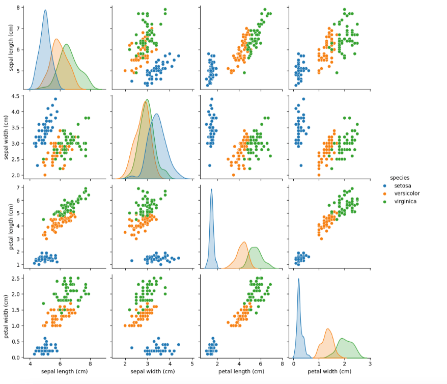
Exploring the dataset visually helps understand the relationships between features and the class distribution. We’ll use scatter plots to visualize the separability of the classes.
import seaborn as sns
import matplotlib.pyplot as plt
# Scatter plot for feature pairs
sns.pairplot(df, hue='species')
plt.show()
Output of the above code:
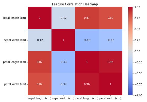
# Correlation heatmap
plt.figure(figsize=(8, 6))
sns.heatmap(df.iloc[:, :-1].corr(), annot=True, cmap='coolwarm', vmin=-1, vmax=1)
plt.title('Feature Correlation Heatmap')
plt.show()
Output of the above code:
Data Preprocessing
Before training the SVM model, we need to preprocess the data by splitting it into training and testing sets and scaling the features.
from sklearn.model_selection import train_test_split
from sklearn.preprocessing import StandardScaler
# Split the data into training and testing sets
X = df.drop('species', axis=1)
y = df['species']
X_train, X_test, y_train, y_test = train_test_split(X, y, test_size=0.3, random_state=42)
# Scale the features
scaler = StandardScaler()
X_train = scaler.fit_transform(X_train)
X_test = scaler.transform(X_test)
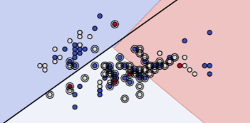
Implementing Support Vector Machine (SVM)
We will use the SVC class from scikit-learn to implement the Support Vector Machine model. We'll start with a basic linear kernel and then explore different kernels to see how they impact the model’s performance.
from sklearn.svm import SVC
from sklearn.metrics import classification_report, accuracy_score
# Initialize and train the SVM model with a linear kernel
svm_model = SVC(kernel='linear', random_state=42)
svm_model.fit(X_train, y_train)
# Make predictions on the test set
y_pred = svm_model.predict(X_test)
# Evaluate the model
accuracy = accuracy_score(y_test, y_pred)
print(f'Accuracy: {accuracy * 100:.2f}%')
# Classification report
print(classification_report(y_test, y_pred))
Output of the above code:
Accuracy: 97.78%
              precision    recall  f1-score   support

      setosa       1.00      1.00      1.00        19
  versicolor       1.00      0.92      0.96        13
   virginica       0.93      1.00      0.96        13

    accuracy                           0.98        45
   macro avg       0.98      0.97      0.97        45
weighted avg       0.98      0.98      0.98        45
Exploring Different Kernels for Support Vector Machine (SVM)
SVM can use different kernels to handle non-linearly separable data. We’ll explore the polynomial and radial basis function (RBF) kernels to compare their performance.
# SVM with polynomial kernel
svm_poly = SVC(kernel='poly', degree=3, random_state=42)
svm_poly.fit(X_train, y_train)
y_pred_poly = svm_poly.predict(X_test)
print(f'Polynomial Kernel Accuracy: {accuracy_score(y_test, y_pred_poly) * 100:.2f}%')
# SVM with RBF kernel
svm_rbf = SVC(kernel='rbf', random_state=42)
svm_rbf.fit(X_train, y_train)
y_pred_rbf = svm_rbf.predict(X_test)
print(f'RBF Kernel Accuracy: {accuracy_score(y_test, y_pred_rbf) * 100:.2f}%')
Output of the above code:
Polynomial Kernel Accuracy: 95.56%
RBF Kernel Accuracy: 100.00%
Conclusion
In this blog, we explored the Iris dataset and implemented a Support Vector Machine (SVM) classifier using Python. We started with a linear kernel and then examined polynomial and RBF kernels to understand their impact on model performance. SVM’s flexibility with different kernels makes it a powerful tool for handling a variety of classification problems. By applying these techniques to the Iris dataset, we gained insights into the effectiveness of SVM for classifying multi-class data and the importance of feature scaling and kernel choice in achieving accurate predictions.
Comments