
Support Vector Machines (SVMs) are a powerful class of supervised learning algorithms used for classification and regression tasks. Known for their ability to handle high-dimensional data and find optimal decision boundaries, SVMs are a popular choice in machine learning. In this blog, we will demonstrate how to implement an SVM classifier on the Diabetes dataset using Python, leveraging the scikit-learn library.

Support Vector Machines (SVM) in Python
Support Vector Machines (SVM) are a robust and versatile set of supervised learning methods used for both classification and regression. Known for their ability to handle high-dimensional data, SVMs work by finding the hyperplane that best separates different classes in the feature space. In Python, Implemented through the scikit-learn library, SVMs aim to find the optimal hyperplane that best separates the data into different classes. By using different kernel functions such as linear, polynomial, and radial basis function (RBF), SVMs can effectively handle linear and non-linear classification problems. In Python, the SVC class is utilized to create and train an SVM model. The process involves loading the dataset, splitting it into training and testing sets, and fitting the model to the training data using the fit() method. Once trained, the model can make predictions on new data, which can be evaluated using metrics like accuracy and classification reports. SVMs are known for their robustness, especially in high-dimensional spaces, and their ability to handle cases where the number of dimensions exceeds the number of samples, making them a valuable tool for various machine learning applications.
Support Vector Machines (SVM)
The core idea behind SVM is to find the optimal hyperplane that maximizes the margin between different classes. The margin is the distance between the hyperplane and the nearest data points from each class, known as support vectors. By maximizing this margin, SVM aims to improve the model's ability to generalize to unseen data.
SVM can handle both linear and non-linear classification tasks. For non-linear data, SVM employs kernel functions, such as polynomial, radial basis function (RBF), and sigmoid, to transform the input space into a higher-dimensional space where a linear separation is possible. Support Vector Machines (SVM) are a set of supervised learning methods used for classification, regression, and outlier detection. The goal of an SVM classifier is to find the optimal hyperplane that maximizes the margin between two classes. SVM is particularly effective in high-dimensional spaces and is versatile due to the use of different kernel functions.
Linear Support Vector Machines (SVM)
A linear SVM aims to find the hyperplane that best separates the data points of different classes. The hyperplane is chosen to maximize the margin, which is the distance between the hyperplane and the nearest data points from both classes, known as support vectors.
Non-Linear Support Vector Machines (SVM)
When the data is not linearly separable, SVM can use kernel functions to map the data into a higher-dimensional space where a linear hyperplane can be used to separate the classes. Common kernels include polynomial, radial basis function (RBF), and sigmoid.
Kernel Trick in Support Vector Machines (SVM)
The kernel trick allows SVM to operate in a high-dimensional, implicit feature space without actually computing the coordinates of the data in that space. Instead, it computes the inner products between the images of all pairs of data in the feature space.
Diabetes Dataset in Python
The Diabetes dataset in Python is a widely used dataset for demonstrating machine learning algorithms, particularly for classification tasks. Available through the scikit-learn library, this dataset contains medical diagnostic measurements such as age, BMI, blood pressure, and serum insulin levels, which are used to predict the presence of diabetes. Each record in the dataset includes these features along with a binary outcome indicating whether the patient has diabetes. The dataset is often utilized for educational purposes and in research to illustrate data preprocessing, feature selection, and the application of various machine learning models. Python, with its robust ecosystem of data manipulation and machine learning libraries like pandas and scikit-learn, provides an ideal environment for exploring and analyzing the Diabetes dataset.The Diabetes dataset, accessible via scikit-learn, consists of several features related to diabetes, including:
Pregnancies: Number of times pregnant
Glucose: Plasma glucose concentration after 2 hours in an oral glucose tolerance test
BloodPressure: Diastolic blood pressure (mm Hg)
SkinThickness: Triceps skin fold thickness (mm)
Insulin: 2-Hour serum insulin (mu U/ml)
BMI: Body mass index (weight in kg/(height in m)^2)
DiabetesPedigreeFunction: Diabetes pedigree function (a function that scores the likelihood of diabetes based on family history)
Age: Age (years)
Outcome: Binary target variable indicating whether the patient has diabetes (1) or not (0)
Implementing Support Vector Machines (SVM) in Python
Implementing Support Vector Machines (SVM) in Python involves using the scikit-learn library to load and preprocess your dataset, split it into training and testing sets, and train the SVM model using the SVC class. The trained model can then be used to make predictions and evaluate performance using metrics such as accuracy and classification reports. SVMs are particularly effective for classification tasks, especially in high-dimensional spaces
Import Libraries
Start by importing the necessary libraries for data manipulation, model training, and evaluation.
import numpy as np
import pandas as pd
from sklearn.datasets import load_diabetes
from sklearn.model_selection import train_test_split
from sklearn.svm import SVC
from sklearn.metrics import accuracy_score, classification_report
import matplotlib.pyplot as plt
Load and Prepare the Data
Load the dataset, preprocess it, and split it into training and testing sets.
# Load the Diabetes dataset
diabetes = load_diabetes()
X = diabetes.data
y = diabetes.target
# Convert the target variable to binary for classification
y_binary = (y > np.median(y)).astype(int)
# Split the dataset into training and testing sets
X_train, X_test, y_train, y_test = train_test_split(X, y_binary, test_size=0.3, random_state=42)
Initialize and Train the SVM Model
Create an SVM model and fit it to the training data.
# Initialize the SVM classifier
clf = SVC(kernel='linear', random_state=42)
# Train the model
clf.fit(X_train, y_train)
Make Predictions and Evaluate the Model
Use the trained model to make predictions on the test set and evaluate its performance.
# Make predictions on the test set
y_pred = clf.predict(X_test)
# Evaluate the model
accuracy = accuracy_score(y_test, y_pred)
print(f'Accuracy: {accuracy * 100:.2f}%')
print('Classification Report:')
print(classification_report(y_test, y_pred))
Output of the above code:
Accuracy: 82.71%
Classification Report:
              precision    recall  f1-score   support

           0       0.85      0.83      0.84        72
           1       0.81      0.82      0.81        61

    accuracy                           0.83       133
   macro avg       0.83      0.83      0.83       133
weighted avg       0.83      0.83      0.83       133
Visualize the Decision Boundary (Optional)
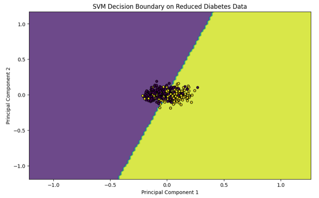
For visualization, you can project the data onto two dimensions if necessary, and plot the decision boundary to understand the classifier's behavior. Note that this step is more complex when dealing with datasets having more than two features.
# For visualization, reduce dimensions to 2 for plotting
from sklearn.decomposition import PCA
X_reduced = PCA(n_components=2).fit_transform(X)
# Split the reduced data
X_train_reduced, X_test_reduced, y_train_reduced, y_test_reduced = train_test_split(X_reduced, y_binary, test_size=0.3, random_state=42)
# Train SVM on reduced data
clf_reduced = SVC(kernel='linear', random_state=42)
clf_reduced.fit(X_train_reduced, y_train_reduced)
# Plot decision boundary
plt.figure(figsize=(10, 6))
h = .02 # step size in the mesh
x_min, x_max = X_reduced[:, 0].min() - 1, X_reduced[:, 0].max() + 1
y_min, y_max = X_reduced[:, 1].min() - 1, X_reduced[:, 1].max() + 1
xx, yy = np.meshgrid(np.arange(x_min, x_max, h),
np.arange(y_min, y_max, h))
Z = clf_reduced.predict(np.c_[xx.ravel(), yy.ravel()])
Z = Z.reshape(xx.shape)
plt.contourf(xx, yy, Z, alpha=0.8)
plt.scatter(X_reduced[:, 0], X_reduced[:, 1], c=y_binary, edgecolor='k', s=20)
plt.title('SVM Decision Boundary on Reduced Diabetes Data')
plt.xlabel('Principal Component 1')
plt.ylabel('Principal Component 2')
plt.show()
Output of the above code:
Full Code for Implementing Support Vector Machines (SVM) on the Diabetes Dataset in Python
Implementing Support Vector Machines (SVM) on the Diabetes dataset in Python involves several key steps: loading the data, preprocessing it, training the SVM model, and evaluating its performance. The process begins by importing necessary libraries such as numpy, pandas, and scikit-learn. The Diabetes dataset is then loaded using load_diabetes() from scikit-learn.datasets. For simplicity, the continuous target variable is converted into a binary classification. The dataset is split into training and testing sets using train_test_split(). An SVM model is initialized with the SVC class, and the training data is used to fit the model. Predictions are made on the test set, and the model's performance is evaluated using metrics like accuracy and a classification report. This comprehensive script provides a step-by-step guide to implementing SVM, showcasing its effectiveness in handling classification tasks on medical data.
Here's the full code:
import numpy as np
import pandas as pd
from sklearn.datasets import load_diabetes
from sklearn.model_selection import train_test_split
from sklearn.svm import SVC
from sklearn.metrics import accuracy_score, classification_report
import matplotlib.pyplot as plt
# Load the Diabetes dataset
diabetes = load_diabetes()
X = diabetes.data
y = diabetes.target
# Convert the target variable to binary for classification
y_binary = (y > np.median(y)).astype(int)
# Split the dataset into training and testing sets
X_train, X_test, y_train, y_test = train_test_split(X, y_binary, test_size=0.3, random_state=42)
# Initialize the SVM classifier with a linear kernel
clf = SVC(kernel='linear', random_state=42)
# Train the model
clf.fit(X_train, y_train)
# Make predictions on the test set
y_pred = clf.predict(X_test)
# Evaluate the model
accuracy = accuracy_score(y_test, y_pred)
print(f'Accuracy: {accuracy * 100:.2f}%')
print('Classification Report:')
print(classification_report(y_test, y_pred))
# Optional: Visualize the decision boundary
# Reduce dimensions to 2 for plotting
from sklearn.decomposition import PCA
X_reduced = PCA(n_components=2).fit_transform(X)
# Split the reduced data
X_train_reduced, X_test_reduced, y_train_reduced, y_test_reduced = train_test_split(X_reduced, y_binary, test_size=0.3, random_state=42)
# Train SVM on reduced data
clf_reduced = SVC(kernel='linear', random_state=42)
clf_reduced.fit(X_train_reduced, y_train_reduced)
# Plot decision boundary
plt.figure(figsize=(10, 6))
h = .02 # step size in the mesh
x_min, x_max = X_reduced[:, 0].min() - 1, X_reduced[:, 0].max() + 1
y_min, y_max = X_reduced[:, 1].min() - 1, X_reduced[:, 1].max() + 1
xx, yy = np.meshgrid(np.arange(x_min, x_max, h),
np.arange(y_min, y_max, h))
Z = clf_reduced.predict(np.c_[xx.ravel(), yy.ravel()])
Z = Z.reshape(xx.shape)
plt.contourf(xx, yy, Z, alpha=0.8)
plt.scatter(X_reduced[:, 0], X_reduced[:, 1], c=y_binary, edgecolor='k', s=20)
plt.title('SVM Decision Boundary on Reduced Diabetes Data')
plt.xlabel('Principal Component 1')
plt.ylabel('Principal Component 2')
plt.show()
Conclusion
Implementing Support Vector Machines (SVM) on the Diabetes dataset in Python demonstrates the versatility and power of SVMs in handling classification tasks, particularly in high-dimensional spaces. By following a structured process that includes loading and preprocessing the dataset, splitting it into training and testing sets, training the SVM model, and evaluating its performance, we can achieve a robust and effective classification model. The use of scikit-learn makes the implementation straightforward, allowing for efficient model training and evaluation. The optional visualization of the decision boundary provides additional insights into the model's behavior. Overall, SVMs prove to be a valuable tool in the machine learning toolkit, capable of delivering accurate predictions and deep insights into complex datasets like the Diabetes dataset. This implementation not only highlights the practical applications of SVM but also reinforces its importance in the field of medical data analysis.
Commenti